PHILIPPE FOREST

Hi! My name is Philippe, and this is my portfolio. I'm interested in neuroscience, music, and recent advances in deep learning. I'm curious, creative, and I try to learn new stuff everyday !
CNN EFFICIENCY OPTIMIZATION
Given that where the latest LLM can have up to 100 trillions parameters, the task of optimizing the efficiency of deep neural networks is becoming more critical now than ever. Some initiatives, such as the Micronet challenge aim to "incentivize the development of efficient models and model compression techniques, as well as providing a forum for more rigorous benchmarking and comparison of existing techniques and for the study of combinations of approaches like sparsity, quantization, distillation, and neural architecture search." As part of a class during my final year at IMT Atlantique, we competed as teams of two in a small scale replication of the challenge, with the objective of attaining at least 90% accuracy on the CIFAR-10 dataset, with a model as efficient as possible. Me and my friend Camille François-Martin teamed up and achieved second best overall, with an accuracy of 90.1% and a total of only 112.000 parameters. This is how we did it.
Architecture of the model
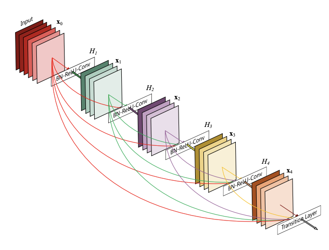
Our final submission will be ranked on a score based on two factors : the number of non-zero parameters and the number of operations necessary to make a full pass through the model. The first one will be highly influenced by the initial model size, or the amout of pruned parameters, whereas the second will moslty be influenced by factors such as quantization, or weight factorization. The first part of the project was obviously chosing our base model architecture. We initially tried with the smallest version of ResNet that we could make, with only 10 convolutional layers, but even this was far too big for our purpose. Instead, we opted for a Densenet architecture. Densenets were introduced in 2016, and exploit the parameter redundancy of classical CNN by connecting the output of every convolutional layer with every other layer of the same simension, thus reducing the need for parameter redundancy. The following image illustrate this principle :
Since the densenet architecture is highly configurable, the question is : how big (or small) should the initial model be? Of course, if we chose a bigger model, we always have the possibility to prune it later, but pruned models typically don't tend to perform as well as unpruned models with the same size. Therefore, it may seem strategic to begin with a model that's already as close as possible to the recquired accuracy treshold (90%), but then we run the risk of dropping below this limit when we are going to apply various techniques to reduce the computation score, such as quantization. This is why it's very important to already have an overview of the various methods we will want to use even before selecting the base model. Thus, we have performed a serie of test in order to see which techniques were promising or not.
Data augmentation and training optimization
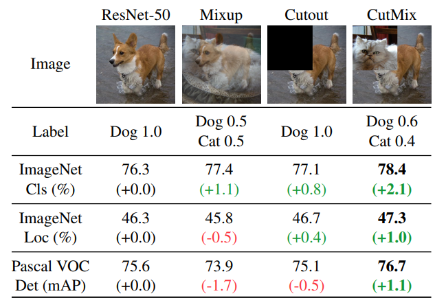
Since our wiggle room is so small with tiny models, we need to make sure that they are used to the best of their capacity. This is why experimenting with various types of data augmentation is crucial is this first step. On top of the classical croping, rotating and jittering techniques that are commonly used, we experimented with a the Mixup algorithm, that allows to effectively "mix" images that belong to two different classes, and their respective labels as well. This approach, combined with a cosine annealing scheduler, and Adam optimizer, allowed us to boost our base accuracy by 1.7% on various Densenet architectures.
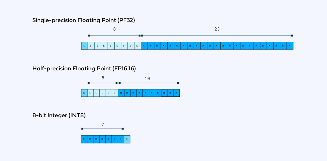
Quantization
Reducing the number of parameters through pruning is one thing, but reducing the number of operations performed during each forward pass is also necessary to acheive a good score in the challenge. The most straightforward way to do so is by performing quantization, which consists in reducing the precision of the weights, biases, and activations such that they consume less memory. There are two different kinds of quantization : for static quantization, the parameters are calculated in advance using a calibration data set. The activations thus have the same precision during each forward pass. For dynamic quantization, the parameters are calculated on-the-fly, and are specific for each forward pass. We experimented with different kinds of quatizations, both static and dynamic, and eventually decided to rely on a 16-bit static quantization, thus dividing the amount of operations performed by two!
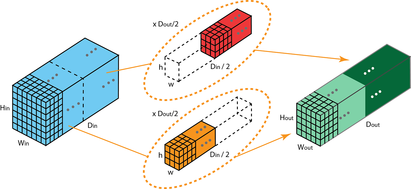
Group convolution
Grouped convolutions is a technique using multiple kernels per layer, resulting in multiple channel outputs per layer. This leads to wider networks allowing to learn richer features with a minimal amount of parameters and operations. When performing a convolution with two groups, the operation becomes equivalent to having two convolutional layers side by side, each seeing half the input channels, and producing half the output channels, and both subsequently concatenated. When performing with as many groups as there are inputs channel, each input channel is convolved with its own set of filters.
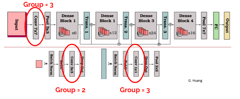
Once again, our experimentation was mostly guided by trial and error, and we eventually settled for 3 grouped convolutions, with size 2, 3 and 3.
Distillation
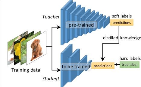
Lastly, we tried to condensate knowledge from a trained Resnet model into our smallest densenet, using the technique of distillation, but to no avail. The basic principle of knowledge distillation involves training the student model to mimic the behavior of the teacher model, rather than directly learning from the training data. This is done by introducing an additional loss term during training, which measures the discrepancy between the output of the teacher model and the student model. During the training phase of the teacher model, an additional output is generated alongside the regular predictions. These additional outputs are called soft targets, and they represent the teacher model's outputs after passing through a softmax function, which converts the outputs into probability distributions over the classes. The student model is then trained on the same dataset used to train the teacher model. However, instead of using the ground truth labels as targets, the soft targets generated by the teacher model are used as guidance for the student model. In addition to the regular loss function used in the student model's training (such as cross-entropy loss), a distillation loss term is introduced. This loss measures the discrepancy between the output probabilities of the student model and the soft targets provided by the teacher model. Therefore, the distillation loss encourages the student model to not only match the teacher model's predictions but also learn from its generalization abilities and fine-grained decision boundaries.
Conclusion
Despite a few shortcomings and a lot of experimentation that did not always go as planned, we eventually managed to finish second of this year, also beating every submissions from last year in the process. If we had more time, we would have liked to experiment with other base architectures such as EfficientNet, or try other kinds of pruning, such as structured pruning, as opposed to the unstructured global pruning that we experimented with.